Display Title
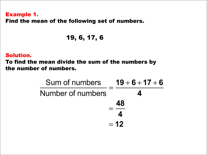
Math Example--Measures of Central Tendency--Mean: Example 1
Display Title
Measures of Central Tendency
Watch this video to learn about sample mean. (The video transcript is included.)
Video Transcript
You’ve seen how normally distributed data have a population mean that is used to construct a probability distribution. In this video we will look at the mean from a random sample of data and how to calculate the mean for the sample.
Let’s start with an example.
A certain species of adult trout has a mean length of 15 inches, with a standard deviation of 2. The table shows a random sample of 30 trout and their length. How does the mean for this data set compare with the population mean?
In this example, we know the mean for the population is 15 inches. Thirty fish are randomly selected for measurement. Do we expect the mean of this data set to be 15?
Realistically, the mean will be close to 15, but we don’t expect it to be exactly the same as the population mean. For that reason, we designate the mean of this data set as the sample mean. It is designated by this formula.
This may look like a new formula, but it’s identical to the mean formula you’ve been working with. The symbol for the sample mean is this and is meant to indicate that it is different from the population mean, mu.
This symbol, the Greek letter sigma, is called the summation symbol. What it says is that we add up all the terms that make up the measurements. In other words, the sum of all the numbers. The denominator is the number of numbers, n. This formula is equivalent to the verbal expression, “the sum of numbers over the number of numbers.”
For this data set, the sample mean is 15.31. As you can see, it isn’t exactly equal to the population mean, but it’s not too far off either.
The standard error of the mean is a measure of how the sample mean differs from the population mean. This is the formula for it. Recall that the symbol sigma is the standard deviation, and n is the number of data items.
For this data set, the standard error is 0.55.
Let’s look at another example.
Adult macaws have an average wingspan of 48 inches, with a standard deviation of 6. The table shows a random sampling of 30 birds whose wingspans were measured. Find the sample mean and the standard error of the mean.
We know the population mean is 48 and we need to find the sample mean based on this data set. This is the formula for finding the sample mean, although you can also use a spreadsheet to calculate it. The sample mean is 46.74.
Now, let’s calculate the standard error. Here is the formula for calculating it. Plug in values for the standard deviation and the number of terms. The standard error comes out to approximately 1.1.
Let’s look at a final example.
Adult male elephants have an average weight of 12,000 pounds, with a standard deviation of 1,500 pounds. The table shows a random sampling of 30 adult male elephants whose weights were measured. Find the sample mean and the standard error of the mean.
The population mean is 12,000 and we need to calculate the sample mean from this data set. You can use the formula to do the calculations, or use a spreadsheet. The sample mean is 12,470.
The standard error is found using this formula. It comes out to 273.86.
Overview
What are Measures of Central Tendency? They are an important way of understanding how data sets cluster. We will be going over the following concepts:
- Mean
- Median
- Mode
- Range
Mean
Suppose you have a data set made up of n terms and suppose the data are arranged in order from least to greatest.:
What is the “average” of this data set? What does it even mean to talk about the average?
Suppose the data are scattered from 0 to 100. Here’s one possible way the data points might cluster:

There are many other ways the data might cluster. The “average” would be the behavior of the data around the middle of the cluster of data.
The term “average” is a general term used to describe this clustering, but there are several mathematical terms that more precisely define this average. The first such term is called the mean.
Using the data set shown earlier (x1…xn), here is the formula for calculating the mean of a data set.

To see some worked-out examples of calculating the mean, click on this link to see a slide show. It includes a video, definitions, formulas, and examples.
The data set for calculating the mean can include negative numbers. To see some worked-out examples of calculating the mean when there are negative numbers in the data set, click on this link to see a slide show.
Another case to consider is what is called a “weighted average.” Click on this link to watch a slide show that explains weighted average in more detail. This includes a video tutorial on weighted averages.
Median
The mean is a very effective, precise way of finding the central tendencies of data sets. But what about when the data sets are huge? For example, if you’ve listened to news reports you’ll often hear about “median household income.” Why not the “mean household income”?
There are millions of people in the data set of “household income.” Going back to our original data set, imagine this data set consisting of millions of data points.
Imagine calculating the mean with this formula with millions of data points:
Do you see the problem? Inputting millions of data points is beyond what a spreadsheet can handle. The number of calculations involved are beyond the abilities of many computers.
So, with extremely large data sets, there’s a different “average” to use, called the median. If you arrange your data set from least to greatest, the median is the term in the middle of the data set.

If there are an odd number of terms, the median is the middle term. For example, the median of five terms is the third term:

If there are an even number of terms, the median is the mean of two of the terms. For example, the median of six terms is the mean of the third and fourth terms.

To see some worked-out examples of finding the median, click on this link to see a slide show. It includes a video, definitions, formulas, and examples.
Mode
A third type of “average” is the mode. It’s especially useful when working with categorical data. For example, suppose you have survey data in which people select their favorite flavor of ice cream. A graph of the data set might look like this.

The mode is the item that occurs most often. The mode can also work with numerical data, but when all you have is categorical data, use the mode.
To see some worked-out examples of finding the mode, click on this link to see a slide show. It includes a video, definitions, formulas, and examples.
Range
Going back to the fictitious data set we’ve been looking at:
If this data set is arranged in order from least to greatest, then the range of values is the difference between the greatest value and the least value.

Special Case: Weighted Average
A particular case of the mean of a data set is what’s referred to as the “weighted average.” This is what such a question would look like:
Look at the following set of coins. What is the average amount of money?

This is an example of a weighted average. If there were only one of each coin, the average, or mean, of the coins would be this:

But the average should take into account that there are three pennies, two dimes, three nickels, and one quarter. This is how to calculate the weighted average:

The numbers in red represent the number or “weight” of each coin. See how the weighted average is lower than the other average calculated? The reason is because of the different number of coins.
|
|


This is a collection of definitions related to measures of central tendency and related concepts. This includes general definitions for mean, median, mode, and range, but also includes definitions for related topics in statistics.
Note: The download is a PNG file.
Related Resources
To see additional resources on this topic, click on the Related Resources tab.
Create a Slide Show
Subscribers can use Slide Show Creator to create a slide show from the complete collection of math definitions on this topic. To see the complete collection of definitions, click on this Link.
To learn more about Slide Show Creator, click on this Link:
Accessibility
This resources can also be used with a screen reader. Follow these steps.
-
Click on the Accessibility icon on the upper-right part of the screen.

-
From the menu, click on the Screen Reader button. Then close the Accessibility menu.

-
Click on the PREVIEW button on the left and then click on the definition card. The Screen Reader will read the definition.
| Common Core Standards | CCSS.MATH.CONTENT.6.SP.B.4, CCSS.MATH.CONTENT.6.SP.A.3, CCSS.MATH.CONTENT.HSS.ID.A.2, CCSS.MATH.CONTENT.HSS.ID.A.3 |
|---|---|
| Grade Range | 6 - 12 |
| Curriculum Nodes |
Algebra • Probability and Data Analysis • Data Analysis |
| Copyright Year | 2014 |
| Keywords | data analysis, tutorials, measures of central tendency, mean, average |